3D GRAFIKA

Zakladni volby, ovlivnujici vzhled 3D grafiky

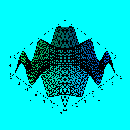
Pouzijeme funkci plot3d a specifikujeme rozsah pro obe promenne.

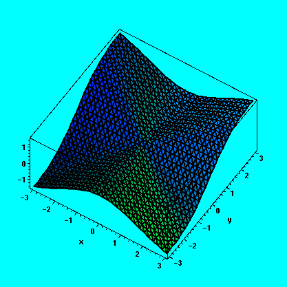
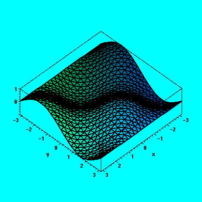
> plot3d(cos(x*y), x=-3..3, y=-3..3);

Obecne plot3d(f(x,y), x=a..b, y=c..d, options);

nebo

plott3d(f, a..b, c..d, options);

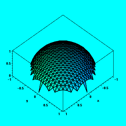
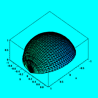
Parametry a,b a c,d nemusi byt vzdy konstantni, srovnejte:

> plot3d(sqrt(1-x^2-y^2),x=-1..1,y=-1..1);

a

> plot3d(sqrt(1-x^2-y^2),x=-1..1,y=-sqrt(1-x^2)..sqrt(1-x^2));

Options muzeme menit i interaktivne z menu.

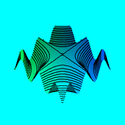
> f:=(x,y)->cos(x*y):

> plot3d(f, -3..3, -3..3, grid=[49,49], axes=boxed, scaling=constrained, style=patchcontour);

Se vsemi options se muzeme seznamit pomoci

> ?plot3d,options

Style:

style=displaystyle

point - pouze kresli pocitane body

line - spojuje body useckami

hidden - i s viditelnosti

wireframe - dratovy model (neuvazuje se viditelnost)

patch - povrch je vykreslen barevne nebo v odstinech sedi

patchnogrid - barevne zobrazeni, ale bez mrizky

contour - pouze vrstevnice

patchcontour - barevne s vrstevnicemi

Shading:

shading=option

z - barvy jsou voleny podle souradnice z bodu povrchu

xy, xyz - kazda z os ma vlastni barevny rozsah

zhue, zgrayscale - barevne odstiny zavisi na souradnici z

Axes:

axes=none, normal, boxed, framed

Orientation and Projection:

Uhly pohledu jsou nastavovany parametrem orientation=[Theta,fi]. Zvetsovanim uhlu Theta rotujeme obrazek proti smeru hodinovych rucicek. Uhel fi urcuje, kde nad (pod)plochou je umisten pozorovaci bod.

projection=r, kde r je z [0,1], specifikuje vzdalenost pozorovaciho bodu od povrchu.

(0 znamena na povrchu, 1 nekonecne vzdaleny, normalni je 1/2).

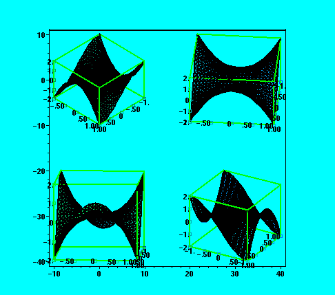
> a:=array(1..2,1..2):

> a[1,1]:=plot3d(x^3-3*x*y^2, x=-1..1, y=-1..1, style=patch, axes=boxed, orientation=[45,45]):

> a[1,2]:=plot3d(x^3-3*x*y^2, x=-1..1, y=-1..1, style=patch, axes=boxed, orientation=[5,45]):

> a[2,1]:=plot3d(x^3-3*x*y^2, x=-1..1, y=-1..1, style=patch, axes=boxed, orientation=[5,80]):

> a[2,2]:=plot3d(x^3-3*x*y^2, x=-1..1, y=-1..1, style=patch, axes=boxed, orientation=[-60,60]):

> plots[display](a);

Zmena stylu osvetlovani nebo zmena pozorovaciho bodu nezpusobi prepocitavani

grafickeho objektu, obrazek se pouze znovu prekresli na obrazovku. Toto vsak neplati pro nasledujici volbu.

Grid:

V 3d nema Maple zjemnovaci algoritmus. Implicitni je mrizka s 25 equidistatntimi body pro oba smery. Toto nastaveni menime parametrem grid=[m,n], m pro osu x, n pro osu y. Pro porovnani vzhledu a vypocetni narocnosti pro ruzne parametry m a n
vyzkousejte nasledujici posloupnost prikazu:

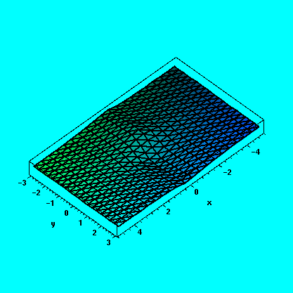
> pp:=(n,m)->plot3d(-y/(1+x^2)/(1+y^2),x=-5..5,y=-3..3,grid=[n,m],style=patch):

> t0:=time():

> pp(20,20);

> t1:=time():

> t1-t0;

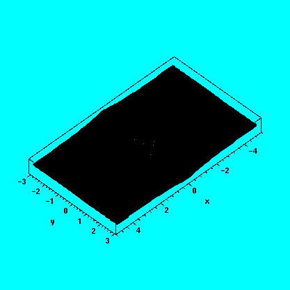
> pp(70,70);

> t2:=time():

> t2-t1;

Pokud by vykresleni nasledujiciho obrazku trvalo prilis dlouho, tak ho preskocte:

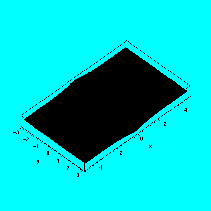
> pp(200,200);

> t3:=time():

> t3-t2;

View Frame:

Podobne jako v 2d muzeme omezit vertikalni rozsah, nebo vsechny rozsahy povrchu pomoci option view.

Pouziva se dvou forem zapisu, bud

view=zmin..zmax

nebo

view=[xmin..xmax, ymin..ymax, zmin..zmax].

Nastaveni pro celou sesion se provadi prikazem setoptions3d.

> plot3d(1/(x^2+y^2), x=-1..1, y=-1..1,axes=boxed);

> plot3d(1/(x^2+y^2), x=-1..1, y=-1..1, view=0..6,axes=boxed);

Struktura grafiky v 3D

Vytvareni grafiky v 3d probiha opet ve dvou fazich (jako v 2d). Nejdrive se pocitaji funkci hodnoty v referencnich bodech, pak je obrazek vykreslovan na obrazovce.

3D graficky objekt v Maplu predstavuje funkce PLOT3D s argumenty popisujicimi osy, funkci, spocitanymi body, parametry mrizky, barvami, atd.

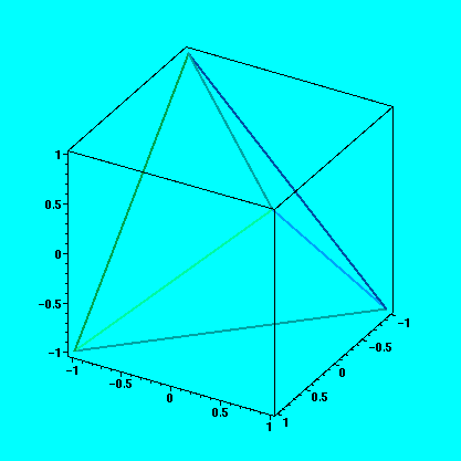
Nasledujici objekt popisuje hrany ctyrstenu s vrcholy (1,1,1), (-1,-1,1), (-1,1,-1) a (1,-1,-1).

> PLOT3D(POLYGONS([ [1,1,1], [-1,-1,1], [-1,1,-1]], [[1,1,1], [-1,-1,1],[1,-1,-1]], [ [-1,1,-1], [1,-1,-1], [-1,-1,1]], [ [-1,1,-1], [1,-1,-1], [1,1,1]]), STYLE(LINE), AXESSTYLE(BOX), ORIENTATION(30,60));

Argumenty(POLYGONS(...), STYLE(...) a AXESSTYLE(...) jsou castmi grafickeho objektu ziskaneho prikazem

> P:=plots[polygonplot3d] ([ [ [1,1,1], [-1,-1,1], [-1,1,-1]], [[1,1,1], [-1,-1,1],[1,-1,-1]], [ [-1,1,-1], [1,-1,-1], [-1,-1,1]], [ [-1,1,-1], [1,-1,-1], [1,1,1]]], style=line, axes=boxed, orientation=[30,60], color=red);

> P;

Obecnejsim prikladem je struktura pro graf funkce x*y^2:

> P:=plot3d(x*y^2, x=-1..1, y=-1..1, grid=[5,5], axes=boxed, orientation=[30,30], style=line, color=black);

> P;

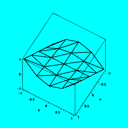
Maple spojuje s funkci dvou promennych na pravouhle siti graficky objekt. Tento objekt je pouzivan pro primkovou interpolaci mezi prilehlymi body obrazku. Funkci hodnoty pro body site jsou pocitany numericky. Neexistuje automaticke zjemnovani site.

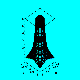
Grafy nespojitych funkci

> f:=(x^2*y)/(x^2+y^2);

> plot3d(f, x=-3..3, y=-3..3, orientation=[-57,38], axes=framed);

Bod, ve kterem vysetrovana funkce neni spojita, je pri teto hustote site totozny s uzlovym bodem a program v nem nemuze
spocitat funkcni hodnotu.

Zmenime hustotu uzlovych bodu tak, aby bod [0,0] (bod nespojitosti) nebyl uzlovym bodem.

> plot3d(f, x=-3..3, y=-3..3, orientation=[-57,38], axes=framed, grid=[30,30]);

Dodefinujeme funkci tak, aby byla spojita.

> g:=proc(x,y) if x=0 and y=0 then 0 else (x^2*y)/(x^2+y^2) fi end:

> plot3d(g, -3..3, -3..3, orientation=[-57,38], axes = framed, labels=[x,y,z]);

Specialni obrazky v 3D

Funkce (krivka) dana parametricky

Prostorove krivky:

> with(plots):

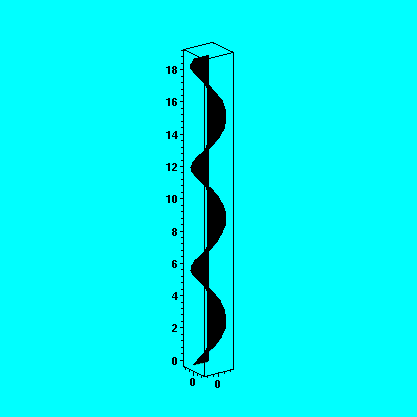
> spacecurve( {[t*cos(2*Pi*t), t*sin(2*Pi*t), 2+t], [2+t, t*cos(2*Pi*t), t*sin(2*Pi*t)], [t*cos(2*Pi*t), 2+t, t*sin(2*Pi*t)]}, t=0..10, numpoints=400, orientation=[40,70], style=line, axes=boxed);

Obecny prikaz pro plochu danou parametricky rovnicemi

x=f(s,t), y=g(s,t), z=h(s,t) je

plot3d([f(s,t), g(s,t), h(s,t)], s=a..b, t=c..d, options);

> plot3d([r*cos(phi), r*sin(phi), phi], r=0..1, phi=0..6*Pi, grid=[15,45], style=patch, orientation=[55,70], shading=zhue, axes=boxed);

Maple podporuje i sfericke a cylindricke souradnice

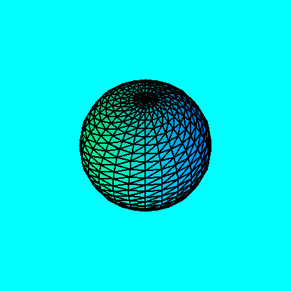
> s:=sphereplot(1, theta=0..2*Pi, phi=0..Pi, style=patch, scaling=constrained): s;

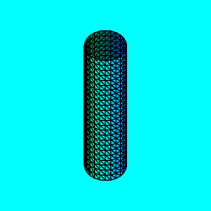
> c:=cylinderplot(1/2, theta=0..2*Pi, z=-2..2, style=patch, scaling=constrained): c;

> display3d({s,c}, style=patchcontour, axes=boxed, orientation=[20,70], scaling=constrained);

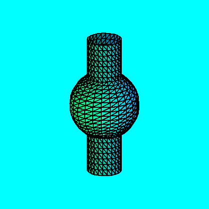
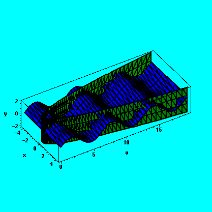
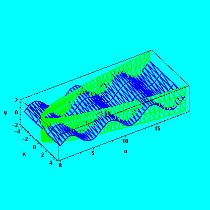
Problemem je zobrazeni prusecnice dvou pronikajicich se povrchu (diky pravouhle mrizce).

> a:=4.4:

> g:=t->t^2:

> h:=sin:

> hz:=plot3d([x,u,sin(u)],x=-a..a,u=0..a^2,color=CYAN,grid=[4,50],

> labels=[x,u,y],axes=frame):

> vt:=plot3d([x,g(x),y],x=-a..a,y=-2..2,grid=[100,4],color=MAGENTA,

> axes=frame,labels=[x,u,y]):

> display3d({hz,vt},orientation=[-32,53]);

> display3d({hz,vt},orientation=[-32,53],style=hidden);

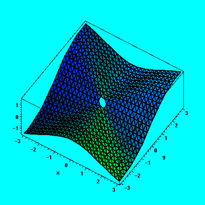
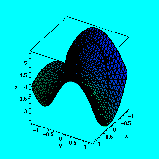
Znazorneni krivky na grafu funkce.

> restart: with(plots):

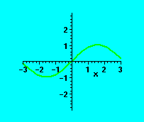
> f:=(x,y)->x^2-y^2+4;

> M:=x^2+y^2=1;

> p1:=plot3d(f(x,y), x=-1.2..1.2, y=-1.2..1.2,axes=framed, orientation=[31,56]):

> p2:=spacecurve([cos(t), sin(t), f(cos(t),sin(t))], t=0..2*Pi, color=black, thickness=3, orientation=[31,56]):

> display3d({p1,p2}, labels=[x,y,z]);

> p4:=spacecurve([cos(t), sin(t), f(cos(t),sin(t))+0.01], t=0..2*Pi, color=black, thickness=3, orientation=[31,56]):

> display3d({p1,p4}, labels=[x,y,z]);

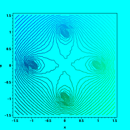
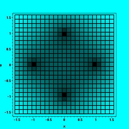
Vrstevnice

contourplot, pocet vrstevnic se nastavuje promennou contours, implicitni nastaveni je 20.

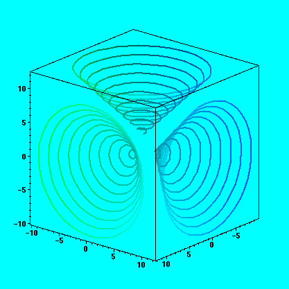
> U:=log(sqrt((x+1)^2+y^2)) + log(sqrt((x-1)^2+y^2)) + log(sqrt((y+1)^2+x^2)) + log(sqrt((y-1)^2+x^2)):

> contourplot(U, x=-3/2..3/2, y=-3/2..3/2, contours=30, numpoints=500, color=black);

> densityplot(U, x=-3/2..3/2, y=-3/2..3/2, numpoints=500, axes=boxed);

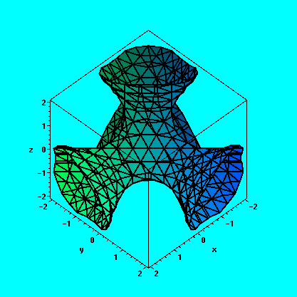
Implicitni funkce

> implicitplot3d( x^3 + y^3 + z^3 + 1 = (x + y +z+1)^3,x=-2..2,y=-2..2,z=-2..2,grid=[13,13,13]);

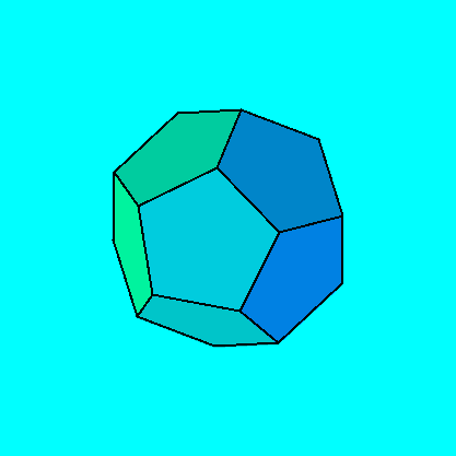
Mnohosteny

(ctyrsten - tetrahedron, osmisten - octahedron, atd.)

> polyhedraplot([0,0,0], polytype=dodecahedron, style=patch, scaling=constrained, orientation=[71,66]);

> ?polyhedraplot

> polyhedra_supported();

Animace

K vytvareni animaci pouzivame prikazu animate ( animate3d ) nebo prikazu display s volbou insequence=true . Pouziti display je obecnejsi a poskytuje vice moznosti.

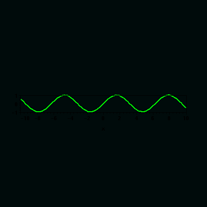
animate( sin(x*t),x=-10..10,t=1..2,frames=50, numpoints=100);

> animate3d(cos(t*x)*sin(t*y),x=-Pi..Pi, y=-Pi..Pi,t=1..2);

> a1:=plot(sin(x), x=-3..3, axes=normal):

> a2:=plot(2*sin(x), x=-3..3, axes=normal):

> a3:=plot(3*sin(x), x=-3..3, axes=normal):

> display({a1,a2,a3},insequence=true);

> a:=k->plot(k*sin(x), x=-3..3, axes=normal):

> display([seq(a(k), k=1..3)], insequence=true);

Prikaz seq slouzi ke generovani posloupnosti podle zadaneho pravidla, syntaxe: seq(vyraz v promenne k , k=rozsah)

> restart:

> with(plots):setoptions(scaling=constrained,axes=none):

> A:=animate([sin(t)+3*k,cos(t)+k^2/4,t=0..2*Pi],k=-5..5,color=blue,thickness=2):

> B:=plot([3*t,t^2/4-1.3,t=-5.5..5.5],color=black,thickness=2):

> display([A,B]);

> restart:

> with(plots):setoptions(scaling=constrained,axes=none):

> a1:=k->plot([sin(t)+3*(5-k),cos(t)+(5-k)^2/4,t=0..2*Pi],color=green,thickness=2):

> a2:=k->plot([sin(t)-3*(15-k),cos(t)+(15-k)^2/4,t=0..2*Pi],color=green,thickness=2):

> a:=proc(k) : if k<11 then a1(k) else a2(k) fi end:

> b:=k->plot([3*t,t^2/4-1.3,t=-5.5..5.5],color=black,thickness=2):

> display([seq(display({a(k),b(k)}),k=1..20)],insequence=true);

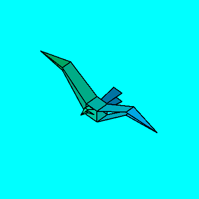
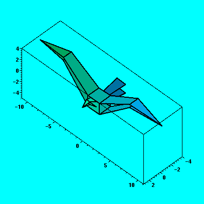
Slozitejsi ukazka animace

> restart:
with(plots):
body := [[1,1,1],[-1,1,1],[-1,-1,1],[1,-1,1]],[[1,1,-1],[-1,1,-1],[-1,-1,-1],[1,-1,-1]],
[[1,1,1],[1,-1,1],[1,-1,-1],[1,1,-1]],[[-1,1,1],[-1,-1,1],[-1,-1,-1],[-1,1,-1]]:
tail:=[[-1,-.5,.5],[-4,-.8,.8],[-4,.8,.8],[-1,.5,.5]],[[-1,-.5,-.5],[-4,-.8,-.8],[-4,.8,-.8],[-1,.5,-.5]]:
lwing01:=[[-1,1,1],[1,1,1],[.5,6,4],[-1,6,4]],[[-1,1,-1],[1,1,-1],[.5,6,3.5],[-1,6,3.5]],
[[.5,6,3.5],[-1,6,3.5],[-.4,11,3],[-.4,11,3]],[[.5,6,4],[-1,6,4],[-.4,11,3],[-.4,11,3]]:
lwing02:=[[-1,1,1],[1,1,1],[.5,6,-2],[-1,6,-2]],[[-1,1,-1],[1,1,-1],[.5,6,-2.5],[-1,6,-2.5]],
[[.5,6,-2.5],[-1,6,-2.5],[-.4,11,-5],[-.4,11,-5]],[[.5,6,-2],[-1,6,-2],[-.4,11,-5],[-.4,11,-5]]:
rwing01:=[[-1,-1,1],[1,-1,1],[.5,-6,4],[-1,-6,4]],[[-1,-1,-1],[1,-1,-1],[.5,-6,3.5],[-1,-6,3.5]],
[[.5,-6,3.5],[-1,-6,3.5],[-.4,-11,3],[-.4,-11,3]],[[.5,-6,4],[-1,-6,4],[-.4,-11,3],[-.4,-11,3]]:
rwing02:=[[-1,-1,1],[1,-1,1],[.5,-6,-2],[-1,-6,-2]],[[-1,-1,-1],[1,-1,-1],[.5,-6,-2.5],[-1,-6,-2.5]],
[[.5,-6,-2.5],[-1,-6,-2.5],[-.4,-11,-5],[-.4,-11,-5]],[[.5,-6,-2],[-1,-6,-2],[-.4,-11,-5],[-.4,-11,-5]]:
head:=[[1,.5,1],[1,-.5,1],[2,-.3,1.5],[2,.3,1.5]],[[1,.5,0],[1,-.5,0],[2,-.3,1],[2,.3,1]],
[[2,-.3,1],[2,.3,1],[3,0,1],[3,0,1]],[[2,-.3,1.5],[2,.3,1.5],[3,0,1],[3,0,1]]:
bird01:=[body,tail,lwing01,rwing01, head]:
bird02:=[body,tail,lwing02,rwing02, head]:
polygonplot3d(bird01, axes = boxed, labels = [x,y,z], scaling=constrained);
polygonplot3d(bird02, axes = boxed, labels = [x,y,z], scaling=constrained);
morph3d:=proc(first,last,t)
local k,j;
[seq([seq([(1-t)*op(1,op(j,op(k,first))) + t*op(1,op(j,op(k,last))),
(1-t)*op(2,op(j,op(k,first))) + t*op(2,op(j,op(k,last))),(1-t)*
op(3,op(j,op(k,first))) + t*op(3,op(j,op(k,last)))],j=1..4)], k=1..nops(first))]:
end:

> a:=seq(polygonplot3d([morph3d(bird01,bird02,t/5)],
scaling = constrained),t=0..5):
b:=seq(polygonplot3d([morph3d(bird02,bird01,t/5)],
scaling = constrained),t=0..5):
display3d([a,b], insequence=true); #try this with the loop button on

Plottools

> restart;

> with(plottools);

> with(plots):

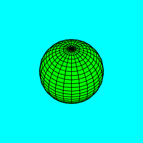
> s1:=sphere([3/2,1/4,1/2], 1/4, color=red):

> display(s1, scaling=constrained);

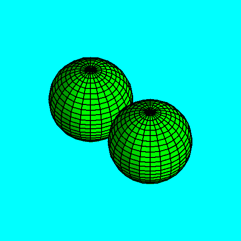
> s2:=sphere([3/2,-1/4,1/2], 1/4, color=red):

> display([s1,s2], axes=normal, scaling=constrained);

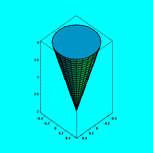
> c:=cone([0,0,2], 1/2, 2, color=khaki):

> display(c, axes=normal);

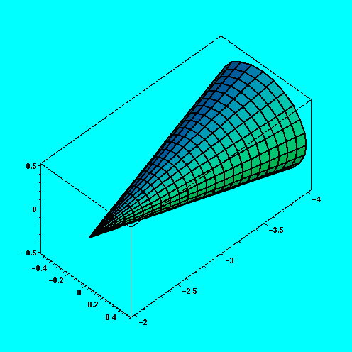
> c2:=rotate(c, 0, Pi/2,0):

> display(c2, axes=normal);

> c3:=translate(c2, 3,0,1/4):

> display(c3, axes=normal);

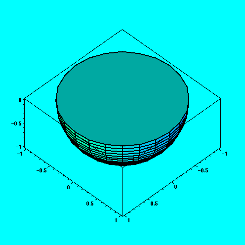
> cup:=hemisphere():

> display(cup);

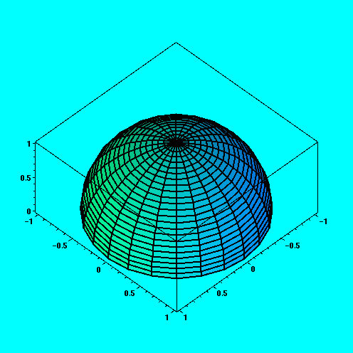
> cap:=rotate(cup, Pi, 0, 0):

> display(cap);

> ?plottools

>

Prezentace na webu pomoci JavaView

> plot2mpl := proc(plot, mpl_file)
local file;
file := fopen(mpl_file, WRITE);
fprintf(file, "%a", plot);
fprintf(file, "%s", ";");
fclose(file);
end;

> objekt:=plot3d(sin(x)*cos(y), x=-3..3, y=-3..3):

> plot2mpl(objekt, `objekt.mpl`);

> save(plot2mpl,`plot2mpl.txt`);

> read(`plot2mpl.txt`);

>